


Visit
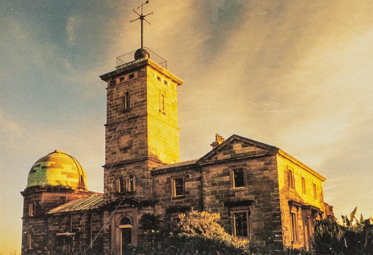
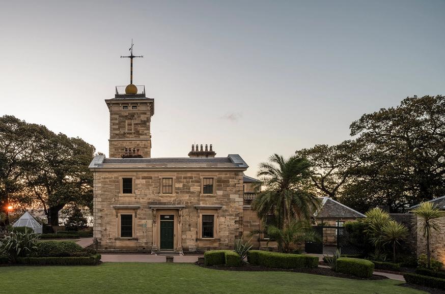
Sydney Observatory
OPEN FOR PRE-BOOKED TOURS AND GENERAL ADMISSION Located on Gadigal land, a national place of connection and scientific research. The site is undergoing heritage conservation works.
Plan Your Visit
Sydney Observatory Map
Sydney Observatory is located on Gadigal land at:
1003 Upper Fort Street, Millers Point, NSW 2000
Powerhouse Museum acknowledges the Gadigal as the Traditional Custodians and the first astronomers of the land Sydney Observatory is situated on. We pay respects to, and seek guidance from, their continuous connection to, and deep knowledge of, the Sky Country above us.
Proudly Supported By

Monthly Sky Guides
Your guide for exploring the Southern night sky. View the latest below.

Stories
A symbol of time and history since 1858, Sydney Observatory has evolved over the years — from steering ships to mapping stars, housing some of Australia's first weather maps to its role now as a public educational space and museum.
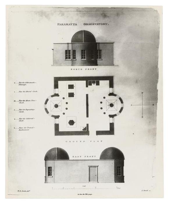
Object No. P3549-44
Photograph of Parramatta Observatory plans used by Sydney Observatory
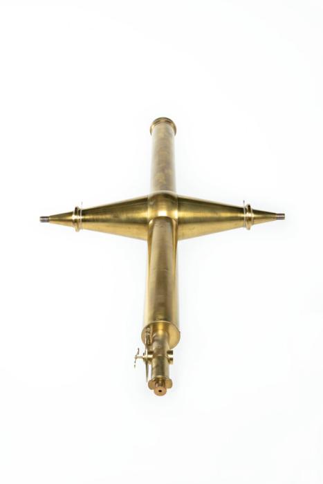
Object No. H9891
Transit telescope made by Edward Troughton
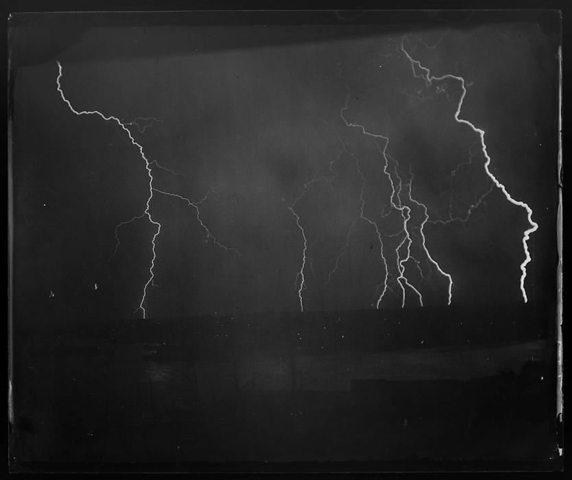
Object No. P3548-783
Photographic glass plate negative, lightning on Sydney suburbs, photographed by H C Russell, Sydney, New South Wales, Australia, 1889-1892
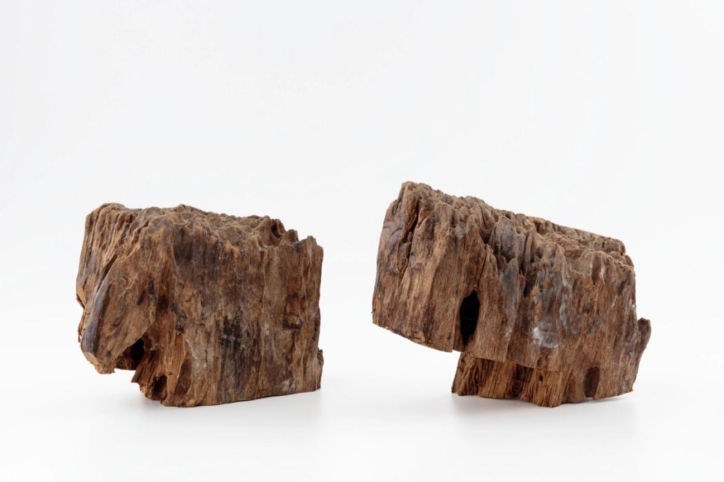
Object No. 2019/38/1
Support posts for the Fort Phillip Signal Station flagstaff
Connect

Opportunity
Opportunities spanning residencies, fellowships, design accelerators and research are offered across all our sites.
More
Community
We support and invest in the development of new work across the applied arts and sciences.
More